


Since the first dice were thrown, roulette wheel was spun, card was drawn, bet was placed or a lottery ticket filled in, humans have sought ways to predict gambling outcomes. And one of those ways has been through math.
Whether you’re playing online casino games or trying your luck at a real brick-and-mortar casino, it’s undeniable that gambling and mathematics have a symbiotic relationship, from designing payment systems for cryptocurrencies and calculating bonuses to calculating probabilities of outcomes occurring in gambling. Gambling, in turn, has been used to develop many mathematical theories. These theories have gone on to be repurposed to solve more complex problems in other fields.
For example, Mathematician Henri Poincaré’s study of the game of roulette fostered his idea of chaos theory, which developed around the turn of the 20th century. Polish scientist Stanislaw Ulam’s experimentation with a variant of solitaire produced the Monte Carlo Method (a modeling method for finding approximate solutions based on random sampling), which is still used today for computer graphics, portfolio management and disease-outbreak analysis.
So what is the relationship between math and gambling?
Mathematics and Gambling
There are arguably two mathematical concepts that are most often used in gambling. These are the concepts of expected value and probability theory. The latter comprises even more concepts.
1. Expected Value

Simply put, expected value is the anticipated value of a bet and is based on how much is bet and how likely the event is to take place.
It represents the average or mean value of the outcomes. The formula is:
E = ∑ [x . P (x) ]
Where E = expected value
∑ = the sum of
x = the amount that can be won/lost
P(x) = probability of a win/loss.
Expected value is used in gambling to predict the average of what one can expect to win or lose in a bet if the bets with identical odds are replicated over a period of time.
Suppose, in a roulette game, the player places a $5 bet on the number 17. There are 38 pockets on this wheel, so they have a 1 in 38 chance of winning.
If the ball lands on 17, the player wins $175 (this is because the standard payout for predicting the correct single number is 1:35.) If not, the house takes the player’s $5. But of course, the roulette ball is far more likely to land on anything other than 17.
What is the expected value of the game to the player?
As per the formula, work out the expected value of a win and the expected value of a loss and add them together.
Win
The probability of a win is 1/38.
[x . P (x) ]
$175 x 1/38 = 4.6053
Loss
The probability of a loss 37/38
-$5 x 37/38 = -4.8684
“Add” those two amounts together.
4.6053 + -4.8684 = -0.2631
You would thus expect to lose an average of 26 cents if you were to make this single-number $5 bet in roulette.
2. Probability Theory
As discussed above, probability theory is at the core of mathematics in gambling. Essentially, when gambling, one is guessing the outcome of an event, which can go several probable ways. Judging whether to place a bet should involve some level of decision as to how likely it is to be successful, which is where probability comes in.
It’s useful to note the different types. Joint probability happens when events occur simultaneously. Marginal probability is the likelihood of an activity taking place irrespective of the results of other events.
Conditional probability is most used in gambling. It’s when the possibility of an event occurring is determined by the occurrence of another mutually exclusive event.
The probability of event X happening given the occurrence of probability Y is expressed as P(X|Y.)
For instance, if one draws a red card from a deck of 52 cards, the probability of that card being a four is P (Four|red) = 2/26 = 1/13.
That is, out of the 26 red cards in the pack, there are two fours.
When two circumstances like X and Y are dependent, the probability of both occurring is: P (X and Y) = P(X) × P (Y given X.)
Conditional probability isn’t cumulative, as clarified by the formula. Bet setters use conditional probability to evaluate the chances of gaining a particular stake given an event has occurred.
The Concept of Permutation
Two ways of working out probability are combinations and permutations.
A permutation is associated with arranging things where the order matters. Combinations are concerned with arranging things where the order does not matter.
When it comes to something like horse racing — where the order of finishing the race matters — you can work out the number of arrangements using a permutation formula.
When it comes to something like the lottery — where the order in which the numbers are drawn does not matter — you can work out the number or arrangements using a combination formula.
Take a look at this using an example:
Suppose one has three letters:
A B C
They can be arranged in other ways::
A C B B A C B C A C A B C B A
There are a total of six permutations (P) of these three letters.
P = 6
However, the number of combinations here is only one.
C = 1
Application of Permutations (Without Repetition) in Horse Racing
Suppose there are four horses that are considered to have an equal chance of winning.
Call them:
A B C D
The next step is to find out all the possible scenarios — or permutations — that these horses could rank (assuming there are no photo-finish ties.)
Start with Horse A coming through as the winner.
ABCD ABDC ACBD ACDB ADBC ADCB
There are six permutations where Horse A comes first, which means there must also be six arrangements where Horse B comes first.
Similarly, there will be six permutations for Horses C and D.
Therefore there are 24 arrangements — or permutations — altogether.
Another way of thinking about this is to choose:
- The first horse in 4 ways (as there are four horses to choose from)
- The second horse in 3 ways (as there are now only three horses to choose from)
- The third horse in 2 ways (as there are now only two horses to choose from)
- The last horse in 1 way (as there is now only one horse to choose from.)
So the number of arrangements = 4 × 3 × 2 × 1 = 24 ways
Another way of showing this is: 4 × 3 × 2 × 1 = 4! (called 4 factorial — the exclamation mark has this special meaning in math)
In general, the number of ways of arranging n distinct (different) objects (where n can be any exact number) is:
n! (n factorial)
n! = n × (n – 1) × (n – 2) × … × 2 × 1
For example:
The number of ways that seven horses could rank is 5,040. See below — the way to calculate this is just like the example with four horses.
7! = 7 × 6 × 5 × 4 × 3 × 2 × 1 = 5,040
The Perfecta/Exacta Bet
A common horse-racing bet is a “perfecta” or “exacta” bet — when you bet on which horses in a race will finish first and second in the exact order.
If there are five horses with an equal chance of winning:
Use the following formula to calculate the number of different permutations possible:
P(n,r) = n! /(n-r)!
where n = the set size (in this instance, the total number of horses)
r = the item select size (the number of horses that must finish in a fixed position)
Applying the formula to the horse race will look like this:
P(5,2) = 5!/(5-2)!
P (5,2) = 5!/3! = 20
This means that there are 20 different possible ways for the horses predicted to place in the first and second place in an exact order to fulfill the parameters of the bet.
To calculate the probability of winning the bet, the number of arrangements that will win the bet must be divided by the total possible number of arrangements of the horses.
To calculate the total number of arrangements possible, use a factorial as seen before (for a five-horse race use 5!):
5! = 5 x 4 x 3 x 2 x 1
= 120
Thus the probability of winning an exacta bet in a race with five horses that have an equal chance of winning (note that this is simplified because in real life there are many factors affecting a horse’s chance of winning) is 20 divided by 120.
ie: 20/120 = 0.166~
or approximately 16.7%.
The Trifecta Bet
Calculating the probability of winning a trifecta bet in horse racing involves considering the number of possible outcomes and the total number of combinations.
First, determine the number of horses participating in the race. Suppose there are “n” horses.
To win a trifecta bet, you need to correctly predict the first, second and third-place finishers in the exact order.
The number of possible outcomes for the first position is “n.” Once the first-place finisher is determined, the number of possible outcomes for the second position is reduced to “n-1” since one horse has already been placed first. Similarly, the number of possible outcomes for the third position becomes “n-2.”
To calculate the probability, divide the number of successful outcomes (winning combinations) by the total number of possible outcomes. The formula is:
Probability = 1 / (n * (n-1) * (n-2))
For example, if there are 10 horses in the race, the probability would be:
Probability = 1 / (10 * 9 * 8) = 1 / 720
Therefore, the probability of winning a trifecta bet in a 10-horse race would be approximately 0.0014 or 0.14%.
If you’d like to learn more about betting, you can read about improving your horse racing betting strategy and a guide to the different kinds of horse racing bets.
Application of Combinations (Without Repetition) Within Lotteries
As discussed, when it comes to combinations, the order of the events does not matter.
Suppose a lottery of 50 numbers has six winning numbers.
The following formula is used to calculate the number of different combinations possible:
C(n,r) = n!/( r! x (n-r)! )
where n = the set size (in this instance, the total number of balls)
r = the item select size (in this case, the winning balls)
Applying the formula to the lottery will look like this:
C(50,6) = 50! / (6! x 44!) = 15,890,700
That means there are 15,890,700 different winning combinations (with none of the numbers repeating,) meaning you have a 1 in 15,890,700 (that’s one in nearly 16 million) chance of winning. When you really break it down like this, it’s easy to see why it’s so rare that six numbers come up.
Combinations in Poker
Another use for combinations would be in casino games such as offline and online poker. Use it to determine the odds of being dealt a royal flush (that’s ace, king, queen, jack, 10 in the same suit) from a single deck of cards.
There are a total of 52 cards in the deck, making the “set” size 52.
n = 52
Deal five cards to a player, making the number of items the player receives from the set 5.
r=5
Applying the formula gives us a total of 2,598,960 possible five-card hands (see below.)
C(52,5) = 52! / (5! x 47!) = 2,598,960
To determine the odds of receiving a royal flush, divide the total number of hands possible by the number of unique royal flushes that can be achieved, which is four (because you can only get one in each suit, of course.) That makes the odds of receiving a royal flush 1 in 649,740.
The Binomial Method
The binomial method of calculating probability, developed by the 17th-century Swiss mathematician Jacob Bernoulli, was a significant step in the development of gambling mathematics.
When considering events with only two possible outcomes (i.e., win or lose,) use binomial probability. It could be tossing a coin, for example.
While determining the probability of one event is simple enough, determining the probability of a specific outcome for a series of events becomes more complicated.
Consider the event of throwing a six-sided dice when you play casino table games. The probability of getting a specific number on a throw is one out of six (i.e., 1/6.)
Use binomial probability to determine the probability of getting two sixes out of five throws.
The formula is as follows:
P (k out of n) = nCk . pk. (1-p)(n-k)
Where n represents the number of trials. In this case, it would be 5.
The number of the specific outcomes, throwing a 6, will be represented by k. The probability of rolling a 6 will be p, whereas (p-1) will be the probability of failing to do so.
n = number of trials
k = number of successes
p = probability of success
1-p = probability of failure
Applying the formula:
P = 5C2 . (16)2(56)3
=
(5!3!2!)(16)2(56)3
=
10(136)(125216)
=
0.16075~
The probability of getting two 6s out of five throws is approximately 0.16 (or 16%.)
Statistics and Gambling
Statistics are used in the analysis of the changes and how lucrative a particular betting activity or market is. Statistics are used by both gamblers and bookmakers as a tool for analysis. Two concepts used are The Law of Large Numbers and Central Limit Theorem.
The Law of Large Numbers

The Law of Large Numbers states, “as the number of identically distributed, randomly generated variables increases, their sample average approaches their theoretical average.”
What does that mean?
Take the simple example of flipping a coin. Theoretically, you have a 50/50 chance of landing on a certain side.
However, if you toss the coin 10 times, you may land heads seven out of the 10 tries, making it 70/30.
But the greater the number of times you flip the coin, the closer the average outcome will be to 50/50.
Simply put, the Law of Large Numbers states that the more often you try, the more likely you are to get an expected outcome — and that outcome relies on the probability of the event taking place.
Central Limit Theorem
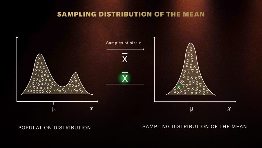
While the Law of Large Numbers states that when a sample size tends to infinity, the sample mean equals the population mean. Central Limit Theorem (CLT) states that when the sample size gets close to a theoretical point of infinity, the sample mean will be normally distributed.
CLT is concerned with the sampling distribution of the mean or average.
Essentially, the Central Limit Theorem allows one to describe how accurately the Law of Averages works.
In order to understand CLT, Box Models must first be understood.
This describes a process in terms of making repeated draws, with replacement, from a box containing numbers.
Since draws are made with replacement, the outcomes in a series of draws are independent. The value on the first draw does not affect the value on the second.
In gambling, box models could describe repeated rolls of a die or repeated tosses of a coin.
Most people have a good intuitive understanding of the Law of Averages, but in many cases, it’s important to determine whether a particular size of deviation between the sample mean and the (usually unknown) expected value is probable or improbable.
That is, what is the chance that the sample average is more than d away from the true EV or expected value?
Formally, the Central Limit Theorem for averages says:

When calculating the chance of winning a given amount of money, use the version of CTL that holds for sums:
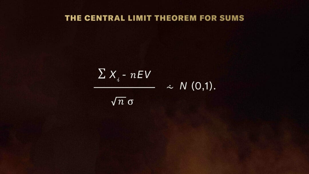
Here, ∑ xi is just the sum of the n drawn from the box.
Here’s how this play out in an example. Say you’re betting on either red or black in roulette. If the ball lands in the color you pick, you win a dollar. Otherwise, you lose a dollar. Suppose you make 100 plays. What is the chance that you lose $10 or more?
First off — what is the box model?
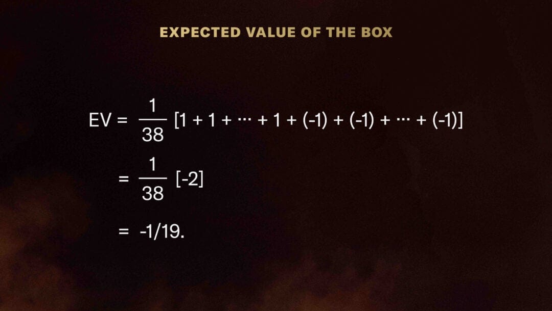
There are 38 objects in the box; 18 are labeled “1” (i.e., you’ll win your dollar) and 20 are labeled “-1” (you’ll lose because only 18 of the 38 slots are your desired color.)
So the expected value of the box is:
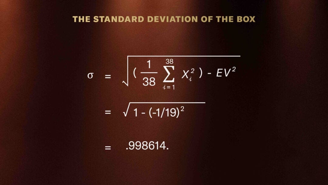
The standard deviation (how different various results are from the average result) of the box is:
The probability of losing more than $10 or more in 100 plays is:
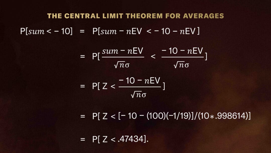
From the standard normal table, the chance of this is about ½ (100 – 34.73)%, so the probability is 0.32635 (or about 33%.)
Calculate Your Way to a Win With BetMGM
While understanding the math may not change how lucky you are when you play online slots or other gambling games, you’ll be able to place bets at your favorite online game casino knowing you’ve got a better idea of the risk you’re taking — and how likely you are to snare a win.
Pit your skills against the house when you register with BetMGM. Go up against a real dealer with live dealer casino games like poker and blackjack at the best live dealer online casino in the US. Looking for the best online slots for real money? BetMGM has some of the biggest jackpot slots on the internet.